 The goal of this class is to help grad students, postdocs, or faculty who have a background in basic statistics and a familiarity with some other statistics package (JMP, SYSTAT, SAS, SPSS) to become comfortable with the R Project as a platform for statistical analyses. It is not meant as a course in statistics, nor does it cover more than a small portion of what is available in R. At the end of the course you should be comfortable managing data in R, making graphs, performing an array of different basic statistical analyses, and be able to use the extensive resources available on line and in books to learn to do just about anything statistical you'd like to in R.
The course is offered periodically, when enough UCSC grad students request it, but you can take the course on your own! The class is primarily based on the handouts below, and videos of the 2015 version lectures are available for UCSC students.
In 2016 I offered a 2-day version of the Transition to R class, covering just the basics to get people up and running in R. Here are the Documents from that class. ENJOY!
RBeginners_A simple analysis.PDF
somedata.csv (Google sheet: File>Download>as CSV file)
IMPORTANT NOTE ON LINKS TO DATA. The website has moved since this course was last offered, so the URLs to datasets in the handouts are broken. Please note, however, that all the datasets are still available, below. You can download them, or get their current URLs by right-clicking on the links, and then modifying the links in the Rcode. I will be updating this soon, but in the meantime...
Plotting resources
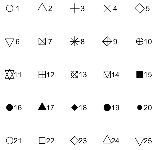
Numbers for plotting symbols; set pch=#
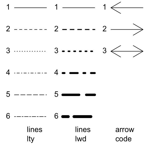
numbers for line type (lty=), line thickness (lwd=) and arrows (code=) for plotting
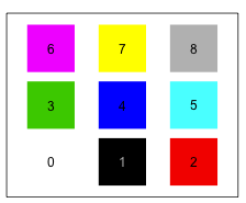
Basic colors called by number for plotting in R (col=)
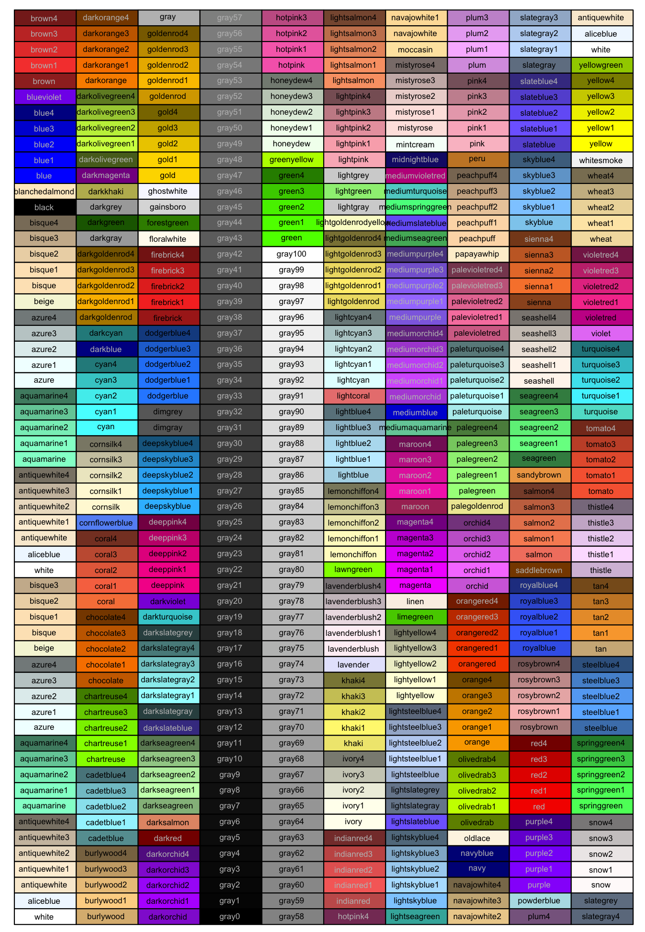
Select colors in R by defined names
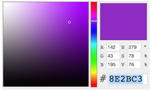
Use the color guide at http://html-color-codes.info to get 6-character color codes, or RGB codes. Then plot(y~x, col="#8E2BC3") or mycol1<-rbg(142/255,43/255,195/255,.7); plot(y~x, pch=19,col=mycol1)
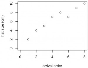 plot(x,y1,xlab="arrival order",ylab="hat size (cm)", ylim=c(0,10),xlim=c(0,8))
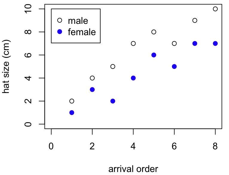 plot(x,y1,xlab="arrival order",ylab="hat size (cm)",ylim=c(0,10),xlim=c(0,8),pch=1,col="black")
points(x,y2,pch=19,col="blue")
legend(0,10,c("male","female"),pch=c(1,19),col=c("black","blue"))

plot(x,y1,xlab="arrival order",ylab="hat size (cm)",ylim=c(0,10),xlim=c(0,8),pch=1,col="black",type="b")
lines(x,y2,pch=19,col="blue",type="o")
#type"p"=points, "l"=lines, "b"= both,"c" lines alone of "b",
#"o" =overplotted,"h"=histogram-like,"s"=stair steps
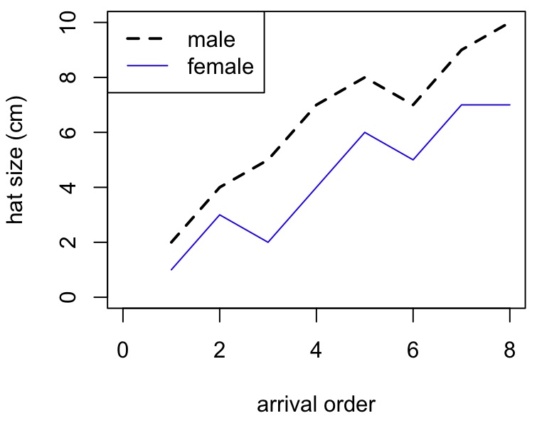 plot(x,y1,xlab="arrival order",ylab="hat size (cm)",ylim=c(0,10),xlim=c(0,8),pch=1,col="black",type="l",lwd=2,lty=2)
lines(x,y2,pch=19,col="blue",type="l",lwd=1,lty=1)
legend("topleft",c("male","female"),lty=c(2,1),col=c("black","blue"),lwd=c(2,1))
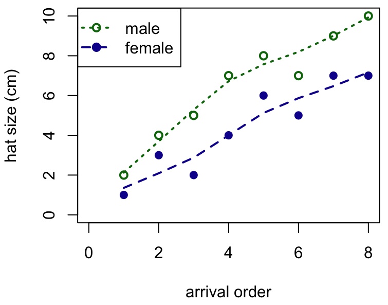 #add smooth lowess curves to each set of points in the scatterplot
plot(x,y1,xlab="arrival order",ylab="hat size (cm)",ylim=c(0,10),xlim=c(0,8),col="dark green",pch=1,lwd=2)
lines(lowess(x,y1),lwd=2,lty=3,col="dark green")
points(x,y2,pch=19,col="dark blue")
lines(lowess(x,y2),lwd=2,lty=2,col="dark blue")
legend("topleft",c("male","female"),lty=c(3,2),pch=c(1,19),col=c("dark green
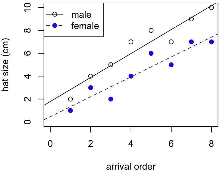 #Use abline to add linear regression lines to each set of points in the scatterplot
plot(x,y1,xlab="arrival order",ylab="hat size (cm)",ylim=c(0,10),xlim=c(0,8),col="black",pch=1,lwd=1)
abline(lm(y1~x),lwd=1,lty=1,col="black")
points(x,y2,pch=19,col="blue")
abline(lm(y2~x),lwd=1,lty=2,col="blue")
legend("topleft",c("male","female"),lty=c(1,2),pch=c(1,19),col=c("black","blue"),lwd=c(1,1))
 #get the relevant statistics for the regression line, then put on the graph as text
a<-summary(lm(y2~x)) #this puts summary stats of the linear regression of y2 on x into list a
R2<-signif(a$adj.r.squared,3) #adjusted R squared
F<-signif(a$fstatistic[1],3) #F statistic
ndf<-signif(a$fstatistic[2],1) #degrees of freedom numerator
ddf<- signif(a$fstatistic[3],1) #degress of freedom denominator
P<-signif(a$coefficients[2,4],4) #P value for significant slope
plot(x,y2,xlab="arrival order",ylab="hat size (cm)",ylim=c(0,10),xlim=c(0,8),col="blue",pch=19,lwd=1)
abline(lm(y2~x),lwd=1,lty=1,col="blue") #puts in the regression line
text(0,9,paste("F=",F,", df=",ndf,",",ddf,"n","R^2=",R2,", P=",P,sep=""),pos=4) #adds the statistics